Introduction to toolStability

Overview

The package toolStability is part of the publication from (Wang, Casadebaig, & Chen, 2023). The package is a collection of functions which implements eleven methods for describing the stability of a trait in terms of genotype and environment.

The goal of this vignette is to introduce users to these functions and get started in analyzing dataset with interaction between genotype and environment.

Further analysis for original publication using this package can be found in the link ( click).

Installation

The package can be installed using the following functions:

# Install from CRAN
install.packages('toolStability', dependencies=TRUE)

# Install development version from Github
devtools::install_github("Illustratien/toolStability")

Then the package can be loaded using the function

library(toolStability)

Welcome to toolStability

This is an r package for calculating parametric, non-parametric, and probabilistic stability indices.

Structure overview of toolStability

toolStability contains different functions to calculate stability indices, including:

adjusted coefficient of variation
coefficient of determination
coefficient of regression
deviation mean squares
ecovalence
environmental variance
genotypic stability
genotypic superiority measure
safety first index
stability variance
variance of rank

Build-in data set

The default data set Data is the subset of \(APSIM\) simulated wheat data set, which includes 5 genotypes in 4 locations for 4 years, with 2 nitrogen application rates, 2 sowing dates, and 2 \(CO_2\) levels of treatments (Casadebaig et al., 2016). Full dataset used in the publication see here click.

Data in this package is a data frame with 640 observations and 8 variables.

Data Structure
Parameters	Number	Description
Trait		Wheat yield (\(kg~ha^{-1}\)).
Genotype	5	varieties.
Environment	128	unique combination of environments for each genotype.
Year	4	years.
Sites	4	locations.
Nitrogen	2	nitrogen application levels.
\(CO_2\)	2	\(CO_2\) concentration levels.
Sowing	2	sowing dates.

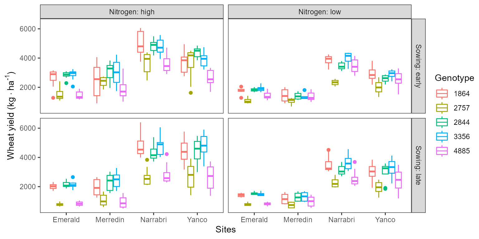
Example of environmental effects on wheat yield.

Tutorial

Data preparation

In order to calculate stability index, you will need to prepare a data frame with 3 columns containing trait, genotype, and environment.

trait: numeric and continuous, trait value to be analyzed.
genotype: character or factor, labeling different genotypic varieties.
environment: character or factor, labeling different environments.

Input formats of function

Most of the functions in the package work with the following format:

function(data = Data,
  trait = "Trait_Column_Name",
  genotype = "Genotype_Column_Name",
  environment = "Environment_Column_Name")

For calculation of probabilistic stability index safety_first_index, an additional parameter lambda is required.

lambda: minimal acceptable value of trait that the user expected from crop across environment. lambda should between the range of trait value.

Under the assumption of trait is normally distributed, safety first index is calculated based on the probability of trait below lambda across the environment for each genotype.

Function Features

Functiontable_stability generates the summary table containing all the stability indices in the package for every genotypes, also including the mean trait value and normality check results for the trait of each genoytpe across all the enviornment.

User can specify the interested combination of environments by entering a vector of column names which containing environmental factors. Option normalize = TRUE allow user to compare between different stability indices. Option unit.correct = TRUE is designed for getting the square root value of stability indices which have the squared unit of trait. For function ecovalence, option modify = TRUE takes the number of environments into account and make modified ecovalence comparable between different number of environments.

Examples

rm(list=ls())
library(toolStability)
### load data
data("Data")
### check the structure of sample dataset
### be sure that the trait is numeric!!!



dplyr::glimpse(Data)
#> Rows: 640
#> Columns: 8
#> $ Genotype    <fct> 1864, 1864, 1864, 1864, 1864, 1864, 1864, 1864, 1864, 1864~
#> $ Yield       <dbl> 1278.6, 1746.0, 1753.9, 1851.8, 2176.6, 2783.3, 3113.3, 27~
#> $ Environment <fct> 1959 Emerald low control early, 1960 Emerald low control e~
#> $ Years       <int> 1959, 1960, 1961, 1962, 1959, 1960, 1961, 1962, 1959, 1960~
#> $ Sites       <fct> Emerald, Emerald, Emerald, Emerald, Yanco, Yanco, Yanco, Y~
#> $ Nitrogen    <fct> low, low, low, low, low, low, low, low, low, low, low, low~
#> $ CO2         <fct> control, control, control, control, control, control, cont~
#> $ Sowing      <fct> early, early, early, early, early, early, early, early, ea~

### calculate ecovalence for all genotypes
single.index.ecovalence <- ecovalence(data = Data,
                                      trait = 'Yield',
                                      genotype = 'Genotype',
                                      environment = 'Environment',
                                      unit.correct = FALSE,
                                      modify = FALSE)
### check the structure of result
dplyr::glimpse(single.index.ecovalence)
#> Rows: 5
#> Columns: 3
#> $ Genotype   <fct> 1864, 2757, 2844, 3356, 4885
#> $ Mean.Yield <dbl> 2878.070, 1913.365, 2911.395, 3038.426, 2024.919
#> $ ecovalence <dbl> 17802705, 27718900, 9365241, 12698454, 24133596

### calculate modified ecovalence for all genotypes
single.index.ecovalence.modified <- ecovalence(data = Data,
                                      trait = 'Yield',
                                      genotype = 'Genotype',
                                      environment = 'Environment',
                                      unit.correct = FALSE,
                                      modify = TRUE)
### check the structure of result
dplyr::glimpse(single.index.ecovalence.modified)
#> Rows: 5
#> Columns: 3
#> $ Genotype            <fct> 1864, 2757, 2844, 3356, 4885
#> $ Mean.Yield          <dbl> 2878.070, 1913.365, 2911.395, 3038.426, 2024.919
#> $ ecovalence.modified <dbl> 139083.63, 216553.91, 73165.94, 99206.67, 188543.72

### calculate all stability indices for all genotypes
summary.table <- table_stability(data = Data,
                                 trait = 'Yield',
                                 genotype = 'Genotype',
                                 environment = 'Environment',
                                 lambda = median(Data$Yield),
                                 normalize = FALSE,
                                 unit.correct = FALSE)
#> Warning in table_stability(data = Data, trait = "Yield", genotype = "Genotype", : 
#> All of your genotypes didn't pass the Shapiro normality test!
#>  Safety_first Index may not be accurate.
#### warning message means your data structure is not distributed as normal distribution

#### check the structure of result
dplyr::glimpse(summary.table)
#> Rows: 5
#> Columns: 15
#> $ Genotype                          <fct> 1864, 2757, 2844, 3356, 4885
#> $ Mean.Yield                        <dbl> 2878.070, 1913.365, 2911.395, 3038.4~
#> $ Normality                         <lgl> FALSE, FALSE, FALSE, FALSE, FALSE
#> $ Safety.first.index                <dbl> 0.3523378, 0.6665326, 0.3242059, 0.2~
#> $ Coefficient.of.determination      <dbl> 0.9398731, 0.8270000, 0.9485154, 0.9~
#> $ Coefficient.of.regression         <dbl> 1.1596475, 0.8552736, 1.0316158, 1.1~
#> $ Deviation.mean.squares            <dbl> 108789.28, 193280.79, 73052.65, 8677~
#> $ Environmental.variance            <dbl> 1809327, 1117230, 1418923, 1630384, ~
#> $ Genotypic.stability               <dbl> 29248135, 24360429, 14583562, 214768~
#> $ Genotypic.superiority.measure     <dbl> 89307.69, 1004043.78, 70091.10, 3048~
#> $ Variance.of.rank                  <dbl> 1.770116, 2.281250, 1.561946, 1.7913~
#> $ Stability.variance                <dbl> 173448.30, 303582.09, 62720.42, 1064~
#> $ Adjusted.coefficient.of.variation <dbl> 50.31578, 47.87130, 44.31829, 46.565~
#> $ Ecovalence                        <dbl> 17802705, 27718900, 9365241, 1269845~
#> $ Ecovalence.modified               <dbl> 139083.63, 216553.91, 73165.94, 9920~

### calculate all stability indices for all genotypes
normalized.summary.table <- table_stability(data = Data,
                                            trait = 'Yield',
                                            genotype = 'Genotype',
                                            environment = 'Environment',
                                            lambda = median(Data$Yield),
                                            normalize = TRUE,
                                            unit.correct = FALSE)
#> Warning in table_stability(data = Data, trait = "Yield", genotype = "Genotype", : 
#> All of your genotypes didn't pass the Shapiro normality test!
#>  Safety_first Index may not be accurate.
#### warning message means your data structure is not distributed as normal distribution

#### check the structure of result
dplyr::glimpse(normalized.summary.table)
#> Rows: 5
#> Columns: 15
#> $ Genotype                          <fct> 1864, 2757, 2844, 3356, 4885
#> $ Mean.Yield                        <dbl> 2878.070, 1913.365, 2911.395, 3038.4~
#> $ Normality                         <lgl> FALSE, FALSE, FALSE, FALSE, FALSE
#> $ Safety.first.index                <dbl> 0.85683453, 0.00000000, 0.93355270, ~
#> $ Coefficient.of.determination      <dbl> 0.07112157, 1.00000000, 0.00000000, ~
#> $ Coefficient.of.regression         <dbl> 0.0000000, 0.9787025, 0.4116811, 0.1~
#> $ Deviation.mean.squares            <dbl> 0.7027599, 0.0000000, 1.0000000, 0.8~
#> $ Environmental.variance            <dbl> 0.0000000, 0.9389617, 0.5296575, 0.2~
#> $ Genotypic.stability               <dbl> 0.0000000, 0.3333003, 1.0000000, 0.5~
#> $ Genotypic.superiority.measure     <dbl> 0.9395799, 0.0000000, 0.9593184, 1.0~
#> $ Variance.of.rank                  <dbl> 0.8095988, 0.3420919, 1.0000000, 0.7~
#> $ Stability.variance                <dbl> 0.5402844, 0.0000000, 1.0000000, 0.8~
#> $ Adjusted.coefficient.of.variation <dbl> 0.0000000, 0.4075840, 1.0000000, 0.6~
#> $ Ecovalence                        <dbl> 0.5402844, 0.0000000, 1.0000000, 0.8~
#> $ Ecovalence.modified               <dbl> 0.5402844, 0.0000000, 1.0000000, 0.8~

### compare the result from summary.table and normalized.summary.table


### calculate the stability indices only based only on CO2 and Nitrogen environments
summary.table2 <- table_stability(data = Data,
                                  trait = 'Yield',
                                  genotype = 'Genotype',
                                  environment = c('CO2','Nitrogen'),
                                  lambda = median(Data$Yield),
                                  normalize = FALSE,
                                  unit.correct = FALSE)
#> Warning in table_stability(data = Data, trait = "Yield", genotype = "Genotype", : 
#> All of your genotypes didn't pass the Shapiro normality test!
#>  Safety_first Index may not be accurate.

#### check the structure of result
dplyr::glimpse(summary.table2)
#> Rows: 5
#> Columns: 15
#> $ Genotype                          <fct> 1864, 2757, 2844, 3356, 4885
#> $ Mean.Yield                        <dbl> 2878.070, 1913.365, 2911.395, 3038.4~
#> $ Normality                         <lgl> FALSE, FALSE, FALSE, FALSE, FALSE
#> $ Safety.first.index                <dbl> 0.3523378, 0.6665326, 0.3242059, 0.2~
#> $ Coefficient.of.determination      <dbl> 0.161086973, 0.138169855, 0.28644744~
#> $ Coefficient.of.regression         <dbl> 1.1791003, 0.8614393, 1.3780191, 1.3~
#> $ Deviation.mean.squares            <dbl> 1517867.6, 962862.6, 1012476.1, 1269~
#> $ Environmental.variance            <dbl> 1809327, 1117230, 1418923, 1630384, ~
#> $ Genotypic.stability               <dbl> 213741097, 130745446, 161091101, 189~
#> $ Genotypic.superiority.measure     <dbl> 3688981, 6251668, 3333615, 3180826, ~
#> $ Variance.of.rank                  <dbl> 2644.454, 1623.286, 2007.764, 2479.2~
#> $ Stability.variance                <dbl> 2025117, 1102709, 1229740, 1636649, ~
#> $ Adjusted.coefficient.of.variation <dbl> 50.31578, 47.87130, 44.31829, 46.565~
#> $ Ecovalence                        <dbl> 192140367, 121852817, 131532582, 162~
#> $ Ecovalence.modified               <dbl> 1501096.6, 951975.1, 1027598.3, 1269~

### compare the result from summary.table and summary.table2
### see how the choice of environments affect the data

Equation of stability indices

Let \(X_{ij}\) represent the observed mean value of the genoptype \(i\) in environment \(j\), and let \(\bar{X_{i.}}\), \(\bar{X_{.j}}\) and \(\bar{X_{..}}\) denote the marginal means of genotype \(i\), environment \(j\) and the overall mean, respectively.

adjusted coefficient variation

Adjusted coefficient of variation (Döring & Reckling, 2018) is calculated based on regression function. Variety with low adjusted coefficient of variation is considered as stable. Under the linear model

\[v_{i} = a + b~m_{i}\] where \(v_{i}\) is the \(log_{10}\) of phenotypic variance and \(m_{i}\) is the \(log_{10}\) of phenotypic mean. \[\widetilde{c_{i}} = \frac{1}{\widetilde{\mu_{i}}} \left [ 10^{(2-b)~ m_{i} +(b-2)~ \bar{m}+v_{i}} \right ] ^{0.5} \times 100 \% \]

coefficient of determination

Coefficient of determination (Pinthus, 1973) is calculated based on regression function. Variety with low coefficient of determination is considered as stable. Under the linear model \[Y_{ij} =\mu + \beta_{i}~ e_{j} + g_{i} + d_{ij}\] <<<<<<< Updated upstream where \(Y_{ij}\) is the predicted phenotypic values, \(g_{i}\), \(e_{j}\) and \(\mu\) denoting genotypic, environmental and overall population mean, respectively. ======= where \(Y_{ij}\) is the observed mean value of \(i^{th}\) genotype in the \(j^{th}\) environment; \(g_{i}\), \(e_{j}\) and \(\mu\) denoting genotypic mean, environmental mean and overall population mean, respectively. >>>>>>> Stashed changes

The effect of GE-interaction may be expressed as: \[(ge)_{ij} = \beta_{i}~ e_{j} + d_{ij}\] where \(\beta_{i}\) is coefficient of regression and \(d_{ij}\) is deviation from regression.

For \(s^{2}_{di}\) and \(S_{xi}^{2}\), see \(deviation~mean~squares\) and \(environmental~ variance\) for details.

Coefficient of determination may be expressed as: \[r_{i}^{2} = 1 - \frac{s_{di}^{2}}{s_{xi}^{2}} \]

where \(X_{ij}\) is the observed phenotypic mean value of genotype \(i\) (i = 1,…, G) in environment \(j\) (j = 1,…,E), with \(\bar{X_{i.}}\) and \(\bar{X_{.j}}\) denoting marginal means of genotype \(i\) and environment \(j\), respectively. \(\bar{X_{..}}\) denote the overall mean of \(X\).

coefficient of regression

Coefficient of regression (Finlay & Wilkinson, 1963) is calculated based on regression function. Variety with low coefficient of regression is considered as stable. Under the linear model \[Y_{ij} =\mu + \beta_{i}~ e_{j} + g_{i} + d_{ij}\] <<<<<<< Updated upstream where \(Y_{ij}\) is the predicted phenotypic values, \(g_{i}\), \(e_{j}\) and \(\mu\) denoting genotypic, environmental and overall population mean, respectively. ======= where \(Y_{ij}\) is the observed mean value of \(i^{th}\) genotype in the \(j^{th}\) environment; \(g_{i}\), \(e_{j}\) and \(\mu\) denoting genotypic mean, environmental mean and overall population mean, respectively. >>>>>>> Stashed changes

The effect of GE-interaction may be expressed as: \[(ge)_{ij} = \beta_{i}~ e_{j} + d_{ij}\] where \(\beta_{i}\) is coefficient of regression and \(d_{ij}\) is deviation from regression.

Coefficient of regression may be expressed as: \[ b_{i}=1 + \frac{\sum_{j}(X_{ij} -\bar{X_{i.}}-\bar{X_{.j}}+\bar{X_{..}}) ~ (\bar{X_{.j}}- \bar{X_{..}})}{\sum_{j}(\bar{X_{.j}}-\bar{X_{..}})^{2}}\]

deviation mean squares

Deviation mean squares (Eberhart & Russell, 1966) is calculated based on regression function. Variety with low stability variance is considered as stable.

Deviation mean squares may be expressed as: \[ s^{2}_{di} = \frac{1}{E-2} \left [ \sum_{j}~(X_{ij} - \bar{X_{i.}}- \bar{X_{.j}} + \bar{X_{..}}^{2}) - (b_{i} - 1)^{2} ~ (\bar{X_{.j}}- \bar{X_{..}})^{2} \right ] \]

ecovalence

Ecovalence (Wricke, 1962) is calculated based on square and sum up the genotype–environment interaction all over the environment. Variety with low ecovalence is considered as stable. Ecovalence is expressed as: \[W_{i} = \sum_{j}~(X_{ij} - \bar{X_{i.}} - \bar{X_{.j}} + \bar{X_{..}}^{2})\] To let \(W_{i}\) comparable between experiments, we also provide the modified ecovalence (\(W_{i}'\)), whcih take the number of environments into account. User can get (\(W_{i}'\)) by setting modify = TRUE.

\[W_{i}' = \frac{\sum_{j}~(X_{ij} - \bar{X_{i.}} - \bar{X_{.j}} + \bar{X_{..}}^{2})}{E-1}\] where \(X_{ij}\) is the observed phenotypic mean value of genotype \(i\) (i = 1,…, G) in environment \(j\) (j = 1,…,E), with \(\bar{X_{i.}}\) denoting marginal means of genotype \(i\).

environmental variance

Environmental variance (Römer, 1917) is calculated by squared and summing up all deviation from genotypic mean for each genotype. The larger the environmental variance of one genotype is, the lower the stability.

\[S_{xi}^{2} = \frac{\sum_{j}~(X_{ij} - \bar{X_{i.}})^{2}}{E-1} \] where \(X_{ij}\) is the observed phenotypic mean value of genotype \(i\) (i = 1,…, G) in environment \(j\) (j = 1,…,E), with \(\bar{X_{i.}}\) denoting marginal means of genotype \(i\).

genotypic stability

Genotypic stability (Hanson, 1970) is calculated based on regression function. Variety with low stability variance is considered as stable. Under the linear model \[Y_{ij} =\mu + \beta_{i}~ e_{j} + g_{i} + d_{ij}\] <<<<<<< Updated upstream where \(Y_{ij}\) is the predicted phenotypic values, \(g_{i}\), \(e_{j}\) and \(\mu\) denoting genotypic, environmental and overall population mean, respectively. ======= where \(Y_{ij}\) is the observed mean value of \(i^{th}\) genotype in the \(j^{th}\) environment; \(g_{i}\), \(e_{j}\) and \(\mu\) denoting genotypic mean, environmental mean and overall population mean, respectively. >>>>>>> Stashed changes

The effect of GE-interaction may be expressed as: \[(ge)_{ij} = \beta_{i}~ e_{j} + d_{ij}\] where \(\beta_{i}\) is coefficient of regression and \(d_{ij}\) is deviation from regression.

Genotypic stability: \[ D_{i}^{2} = \sum_{j}~(X_{ij} - \bar{X_{i.}}- b_{min}~ \bar{X_{.j}} + b_{min}~ \bar{X_{..}})^{2}\]

\(b_{min}\) is the minimum value of coefficient of regression over all environments.

genotypic superiority measure

Genotypic superiority measure (Lin & Binns, 1988) is calculatd based on means square distance between maximum value of environment j and genotype i. Variety with low genotypic superiority measure is considered as stable.

\[P_{i} = \sum_{j}^{n} \frac{(X_{ij}-M_{j})^{2}}{2n}\] where \(X_{ij}\) stands for observed trait and \(M_{j}\) stands for maximum response among all genotypes in the \(j^{th}\) location.

safety first index

Safety-first index (Eskridge, 1990) is calculated based on the normality assumption of trait over the environments. Among different environments, trait below a given critical level \(\lambda\) is defined as failure of trait. Safety-first index calculating the probability of trait failure over the environment. Variety with low safety first index is considered as stable.

\[Pr~(Y_{ij} < \lambda) = \Phi \left[ (\lambda - \mu_{i})/ \sqrt \sigma_{ii} \right]\]

where \(\lambda\) is the minimal acceptable value of trait that the user expected from crop across environments. Lambda should between the range of trait value. \(\Phi\) is the cumulative distribution function of the standard normal distribution. \(\mu_{i}\) and \(\sigma_{ii}\) is the mean and variance of the system i. Under the assumption of trait is normally distributed, safety first index is calculated based on the probability of trait below lambda across the environments for each genotype.

stability variance

Stability variance (Shukla, 1972) is calculated based on linear combination of ecovalence and mean square of genotype-environment interaction. Variety with low stability variance is considered as stable.

\[ \sigma^{2}_{i} = \frac{1}{(G-1) ~ (G-2) ~ (E-1)} \left [ G ~(G-1)~ \sum_{j}~(X_{ij} - \bar{X_{i.}}-\bar{X_{.j}} + \bar{X_{..}})^{2}- \sum_{i} \sum_{j}~(X_{ij} - \bar{X_{i.}}-\bar{X_{.j}} + \bar{X_{..}})^{2} \right ] \] where \(X_{ij}\) is the observed phenotypic mean value of genotype \(i\) (i = 1,…, G) in environment \(j\) (j = 1,…,E), with \(\bar{X_{i.}}\) and \(\bar{X_{.j}}\) denoting marginal means of genotype \(i\) and environment \(j\), respectively. \(\bar{X_{..}}\) denote the overall mean of \(X\).

Negative values of stability variance is replaced with 0.

variance of rank

Variance of rank (Nassar & Hühn, 1987) is calculated based on regression function. Variety with low variance of rank is considered as stable.

Correction for each genotype \(i\) was done by subtraction of marginal genotypic mean \(\bar{X_{i.}}\) and the addition of overall mean \(\bar{X_{..}}\). \[X_{corrected~ij} = X_{ij} - \bar{X_{i.}} + \bar{X_{..}}\] Then calculated the rank all genotypes for each environment \(j\) \[r_{ij} = rank~(X_{correctedij})\]

Variance of rank is calculated as the following equation. \[S_{i}4 = \frac{\sum_{j}~(r_{ij}-\bar{r_{i.}})^{2}}{E-1}\] where \(r_{ij}\) is the rank of genotype \(i\) in environment \(j\) and \(\bar{r_{i.}}\) is the marginal rank of genotype \(i\) over environment, based on the corrected \(X_{ij}\) values.

Citing `toolStability`

Wang, TC., Casadebaig, P. & Chen, TW. More than 1000 genotypes are required to derive robust relationships between yield, yield stability and physiological parameters: a computational study on wheat crop. Theor Appl Genet 136, 34 (2023). https://doi.org/10.1007/s00122-023-04264-7

relavant links

* Reproducible R code for publication https://github.com/Illustratien/Wang_2023_TAAG
* Data https://doi.org/10.5281/zenodo.4729636

References

Casadebaig, P., Zheng, B., Chapman, S., Huth, N., Faivre, R., & Chenu, K. (2016). Assessment of the Potential Impacts of Wheat Plant Traits across Environments by Combining Crop Modeling and Global Sensitivity Analysis. PLOS ONE, 11(1), e0146385. https://doi.org/10.1371/journal.pone.0146385

Döring, T. F., & Reckling, M. (2018). Detecting global trends of cereal yield stability by adjusting the coefficient of variation. European Journal of Agronomy, 99, 30–36. https://doi.org/10.1016/j.eja.2018.06.007

Eberhart, S. A., & Russell, W. A. (1966). Stability parameters for comparing varieties. Crop Science, 6(1), 36–40. https://doi.org/10.2135/cropsci1966.0011183X000600010011x

Eskridge, K. M. (1990). Selection of Stable Cultivars Using a Safety-First Rule. Crop Science, 30(2), 369. https://doi.org/10.2135/cropsci1990.0011183X003000020025x

Finlay, K. W., & Wilkinson, G. N. (1963). The analysis of adaptation in a plant-breeding programme. Australian Journal of Agricultural Research, 14(6), 742–754. https://doi.org/10.1071/AR9630742

Hanson, W. D. (1970). Genotypic stability. Theoretical and Applied Genetics, 40(5), 226–231. https://doi.org/10.1007/BF00285245

Lin, C. S., & Binns, M. R. (1988). A superiority measure of cultivar performance for cultivar \(\times\) location data. Canadian Journal of Plant Science, 68(1), 193–198. Retrieved from https://cdnsciencepub.com/doi/10.4141/cjps88-018

Nassar, R., & Hühn, M. (1987). Studies on estimation of phenotypic stability: Tests of significance for nonparametric measures of phenotypic stability. Biometrics, 43(1), 45–53.

Pinthus, M. J. (1973). Estimate of genotypic value: A proposed method. Euphytica, 22(1), 121–123. https://doi.org/10.1007/BF00021563

Römer, T. (1917). Sind die ertragdreichen Sorten ertagissicherer? Mitteilungen Der Deutschen Landwirtschaftlichen Gesellschaft, 32(1), 87–89.

Shukla, G. K. (1972). Some statistical aspects of partitioning genotype environmental components of variability. Heredity, 29(2), 237–245.

Wang, T.-C., Casadebaig, P., & Chen, T.-W. (2023). More than 1000 genotypes are required to derive robust relationships between yield, yield stability and physiological parameters: A computational study on wheat crop. Theoretical and Applied Genetics, 136, 34.

Wricke, G. (1962). Über eine Methode zur Erfassung der ökologischen Streubreite in Feldversuchen. Zeitschrift Für Pflanzenzüchtung, 47, 92–96.

Tien-Cheng Wang

2023-03-10

Overview

Installation

Welcome to toolStability

Structure overview of toolStability

Build-in data set

Tutorial

Examples

Equation of stability indices

adjusted coefficient variation

coefficient of determination

coefficient of regression

deviation mean squares

ecovalence

environmental variance

genotypic stability

genotypic superiority measure

safety first index

stability variance

variance of rank

Citing `toolStability`

relavant links

References

Introduction to toolStability

Tien-Cheng Wang

2023-03-10

Overview

Installation

Welcome to toolStability

Structure overview of toolStability

Build-in data set

Tutorial

Examples

Equation of stability indices

adjusted coefficient variation

coefficient of determination

coefficient of regression

deviation mean squares

ecovalence

environmental variance

genotypic stability

genotypic superiority measure

safety first index

stability variance

variance of rank

Citing toolStability

relavant links

References

Citing `toolStability`