Week3: dataframe and ggplot2

R-basic

Author

Tien-Cheng

Welcome to the third course! You will learn ggplot and dataframe wrangling:

Learning goals

data frame wrangling with dplyr
ggplot2

0.1 practice dataframe with real data

df <- data.frame(time=as.Date("2023-04-16",format="%Y-%m-%d")+seq(1,3,1),
                 temp=c(20,15,13), 
                 thermal_time=cumsum(c(20,15,13)))
df %>% dplyr::glimpse() 
names(df)
# extract column from dataframe
df$thermal_time
df[,3]
df[,'thermal_time']
df[['thermal_time']]

# not work
df[thermal_time]
# different error message
#!! name space conflict
df[time]
time

# summarize dataframe
lapply(df, range)
# turn as data frame
lapply(df, range) %>% data.frame()

summary(df)

Note

Practice with large data set ear_summarized.csv in folder data.

read the file with relative path using function read.csv().
find the row and column number of data frame by nrown() and ncol()
check the range of each column using lapply(), how many unique days exist in column date? check unique()
compare the result of glimpse() and str()
extract column weight using [],[[]]and $ ¹
what is the function of head() and tail()?
how to extract the first three row using []?

¹ You can subset dataframe by indexing [row,column] dataframe[,column] select the whole role for selected columnn dataframe[row,] select the whole column of selected rows

1 dplyr

1.1 Subset row(s)

dplyr::filter(): extract row where the condition matched. ²

² r_package::function_name specify the function name by package name.:: has similar meaning like “from”. It is useful to avoid name space conflict when same function name is used by multiple library that you are using.

e.g., extract temp where time is 2023-04-17 in df.

# df$time %>% str()
df %>% dplyr::filter(time=='2023-04-17') %>% .$temp
df %>% dplyr::filter(time==as.Date('2023-04-17')) %>% .$temp

1.2 Add column(s)

dplyr::mutate(): add one or multiple columns to dataframe.

e.g., add columnYear to df, its value is '2023'.

# result is not save
df %>% dplyr::mutate(Year="2023") 
df
# result is saved
df$Year <- "2023"
df[['Year']] <- "2023"
df

Note

How to save result using %>%? Check example with ?mutate.

1.3 Combine dataframes by column.

df <- data.frame(time=as.Date("2023-04-16",format="%Y-%m-%d")+seq(1,3,1),
                 temp=c(20,15,13), 
                 thermal_time=cumsum(c(20,15,13)))
# with same length dataframe
ear_df <- data.frame(time=as.Date("2023-04-16",format="%Y-%m-%d")+seq(1,3,1),
                     ear_weight=c(20,40,50))
merge(df,ear_df,by="time")
dplyr::left_join(df,ear_df,by="time")
# combind with vector of same length 
cbind(df, ear_weight=c(20,40,50))
df$ear_weight <- c(20,40)

# with differnt length 
short_ear_df <- data.frame(time=as.Date("2023-04-16",format="%Y-%m-%d")+seq(1,2,1),
                           ear_weight=c(20,40))
merge(df,short_ear_df,by="time")
dplyr::left_join(df,short_ear_df,by="time")

# combind with vector of different length 
cbind(df, ear_weight=c(20,40))
df$ear_weight <- c(20,40)

Note

Check description of merge and left_join, how are they different from each other? What happen if you remove the argument by?

2 GGplot2

2.1 ggplot grammar: layer-wise commands

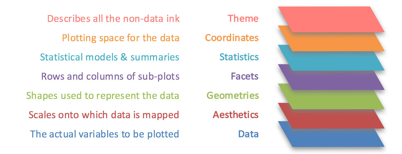
layers of ggplot: click picture for original source

Top layer ggplot()and sub-layers sublayer commands ³, they are separated by +.

³ see function reference for more!

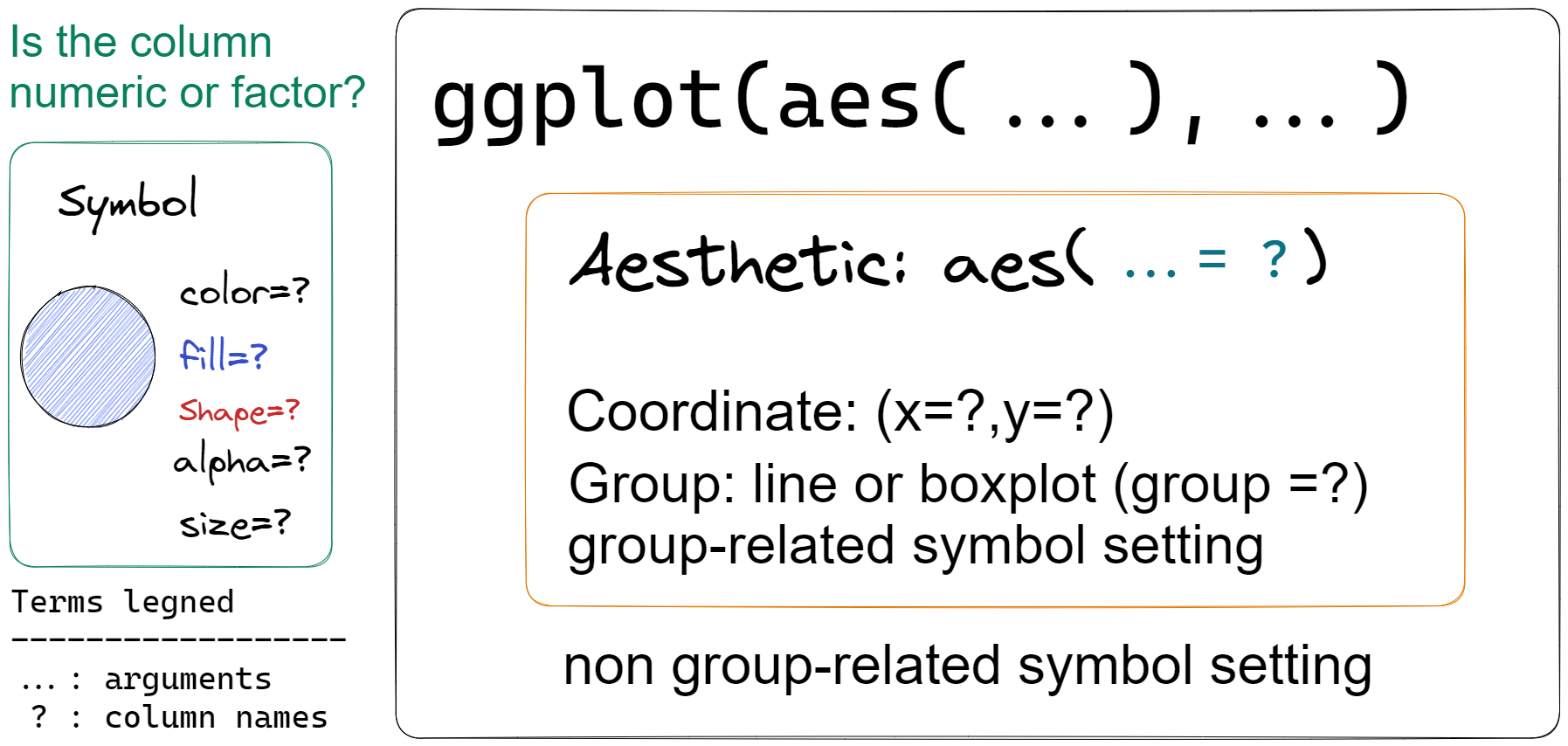
Within each layer, there may be an aesthetic function aes() to set aesthetic setting like x,y and color,fill or shape. Function ggplot() will not generate any graph but used for setting common aesthetic setting across the sub-layer. Plot type are specify in sub-layer with prefix geom_xx.

order matters!

If there are conflicts between the sub-layer commands, the latter will overwrite the previous one!

2.2 Requirements of scientific plot.

axis title: specify with unit if there is any using xlab() or ylab().
legend title: full name instead of default abbreviation using guides().
other important rules: ⁴.

⁴ Ten simple rules for better figures How to Make Good Graphs and Figures for Scientific Papers

# Watch out the names!
library(ggplot)
library(ggplot2)

Note

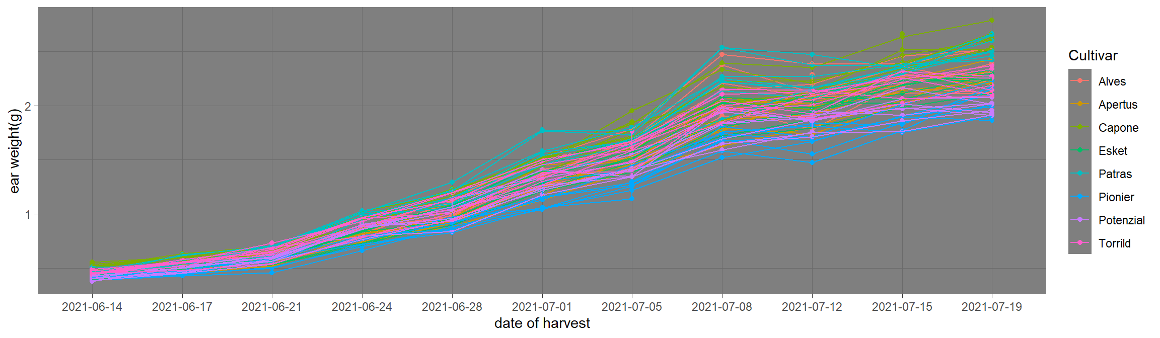
go to HU-box download ear_summarized.csvand put it in folder data. read this file using read.csv with relative path and named it as data

data %>% 
  ggplot(aes(x=date,y=weight,color=var))+
  geom_point()+
  geom_line(aes(group=group))+ # link the point by group.
  xlab("date of harvest")+ #x axis title
  ylab("ear weight(g)")+   #y axis title
  guides(color=guide_legend(title="Cultivar")) #change legend title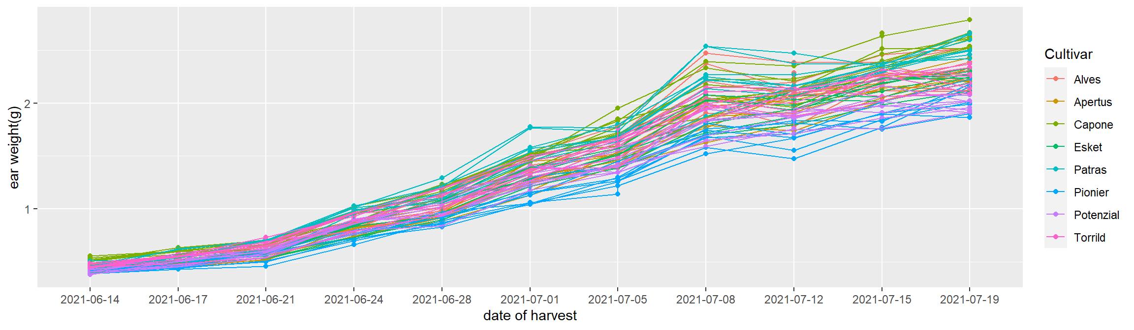

Figure 1: Growth of ear weight over time.

challenge : use theme_xx() function series to change background of the plot. Click for example.

2.3 facet: organized subplot by column

There are two commonly used functionfacet_grid and facet_wrap. In side each function, subplots are arranged in the manner of (row ~ column). There could be multiple column names put in the row or column position.

Note

go to HU-box download phenology_short.csvand put it in folder data. read this file using read.csv with relative path and named it as phenology

phenology %>% 
ggplot(.,aes(x=var,y=value))+
  geom_boxplot()+
  facet_grid(Year~stage)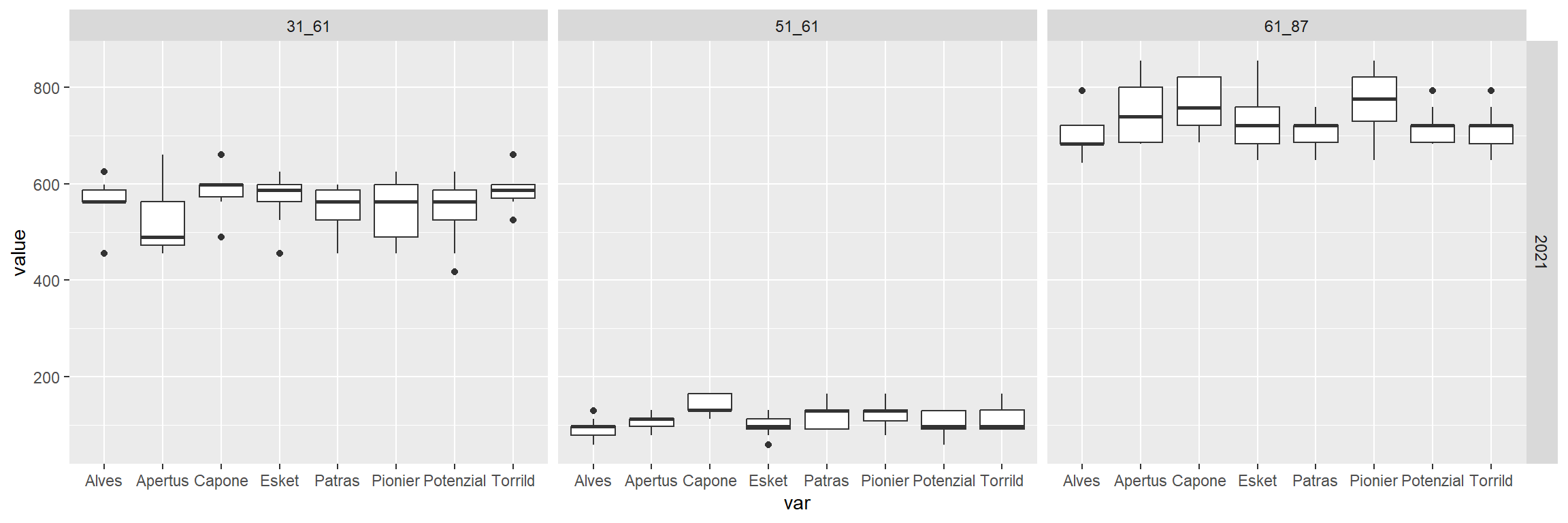

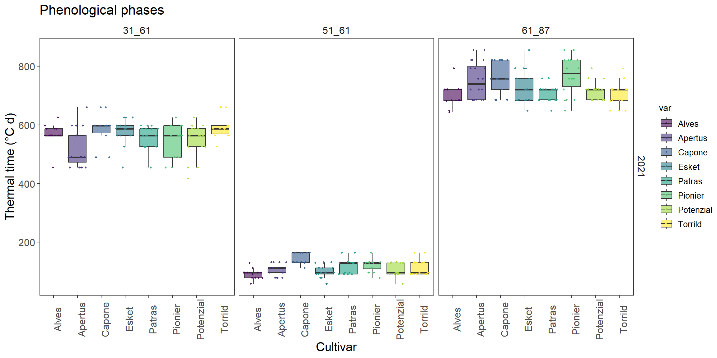
Make this graph more beautiful!

How to make each point show in box plot? (search for scatter points in boxplot ggplot2)

How does color and fill differs? Can you color it by var?

Could you apply another color scale using viridis package?

How to remove the background of the facet title with theme()? what does element_blank() do?

Follow up question, if you also apply theme_test() to it, it should be before or after theme()?

How to change title size? how does it related to element_text()

Could you change the axis title display angle as 90 degree?

How do you add title?

3 Recommendations

3.1 online tutorials:

ggplot datacamp ggplot 2 ggplot gallery

3.2 online books:

ggplot cheatsheet Data visualization with R R for Data Science: Chapter3 Visualization

4 Feedback this week

Anonymous feedback