Week9: Grain development v

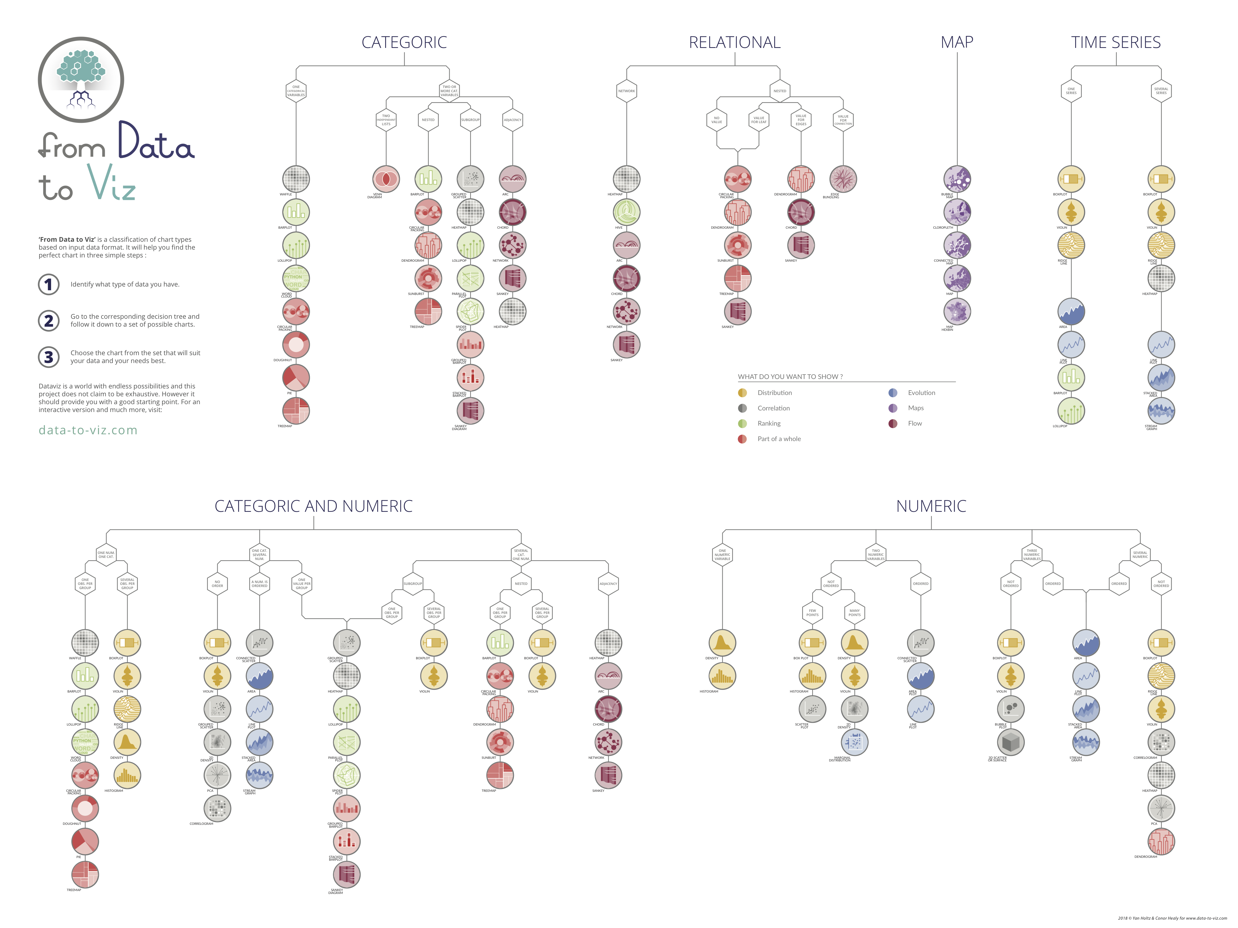
Welcome to the nigth course! You will learn more aboutdata visualization:

Learning goals

1. Warm up for final presentation
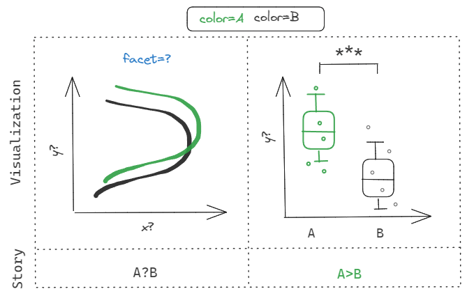
2. Data type based story telling
3. github

Discussion: Warm up for the final presentation!

1. How the shape of dataframe is linked to data visualization?
2. What is the component of for loop? how to examine the function body? Do you need print() to see the result?

range_vector <- 1:10
for( i in range_vector){
  i+3
}

3. What is important when you want to combine the dataframes row-wise?
4. What is the format (columns and data type of columns) of self-collected ear data?
5. Which plot type could be suitable for visualization?
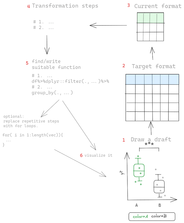
6. What are the logic of visualization oriented analysis? Could you list the possible steps?
7. What are essential elements for reproducible analysis? For example, you have a r script which read the files in the folder and plot a plot.

df <- read.csv("example.csv")
df %>% 
  ggplot() %>% 
  geom_point(aes(x=x,y=y))

Excercise:

1. share your code on github and share it with others.

1 Story telling: Warm up for final Presentation

Figure1: Project Plan

Figure2: Story type

Figure3: Cycle of visualization

Visualization based on data type: click picture for source

^{1 2}

¹ Ten simple rules for better figures

² How to Make Good Graphs and Figures for Scientific Papers

2 Exercise with student’s data

practice with files from data/student.

library(magrittr)
df<- map_dfr(list.files("../data/student"),~{
  
  student_name <-  .x %>% strsplit("_") %>% unlist() %>% 
    .[4] %>% sub(".xlsx","",.)
  
  file<- xlsx::read.xlsx(paste0("../data/student/",.x),sheetIndex = 1) %>%  
    `colnames<-`(stringr::str_to_lower(names(.)))%>% 
    `colnames<-`(gsub("kernal","kernel",names(.))) %>% 
    `colnames<-`(gsub("spikes","spike",names(.)))%>%
    `colnames<-`(gsub("plot.id","plot_id",names(.))) %>% 
    mutate(student=student_name)
}) 
df %<>% mutate(var="Capone",plot_id=159) %>% 
  .[!grepl("na.",names(.))]
df %>% glimpse()

Rows: 57
Columns: 8
$ var          <chr> "Capone", "Capone", "Capone", "Capone", "Capone", "Capone…
$ plot_id      <dbl> 159, 159, 159, 159, 159, 159, 159, 159, 159, 159, 159, 15…
$ spike        <dbl> 1, 2, 3, 4, 5, 6, 7, 8, 9, 10, 11, 12, 13, 14, 15, 16, 17…
$ flower       <dbl> 1, 3, 5, 5, 5, 5, 5, 5, 5, 5, 5, 5, 5, 5, 5, 5, 5, 5, 4, …
$ kernel.full  <dbl> 0, 2, 2, 2, 3, 2, 2, 1, 2, 2, 2, 2, 2, 2, 2, 2, 3, 2, 1, …
$ kernel.half  <dbl> 0, 0, 0, 0, 0, 0, 0, 0, 0, 0, 0, 0, 0, 0, 0, 0, 0, 0, 0, …
$ kernel.small <dbl> 0, 0, 0, 0, 0, 0, 0, 0, 0, 0, 0, 0, 0, 0, 0, 0, 0, 0, 0, …
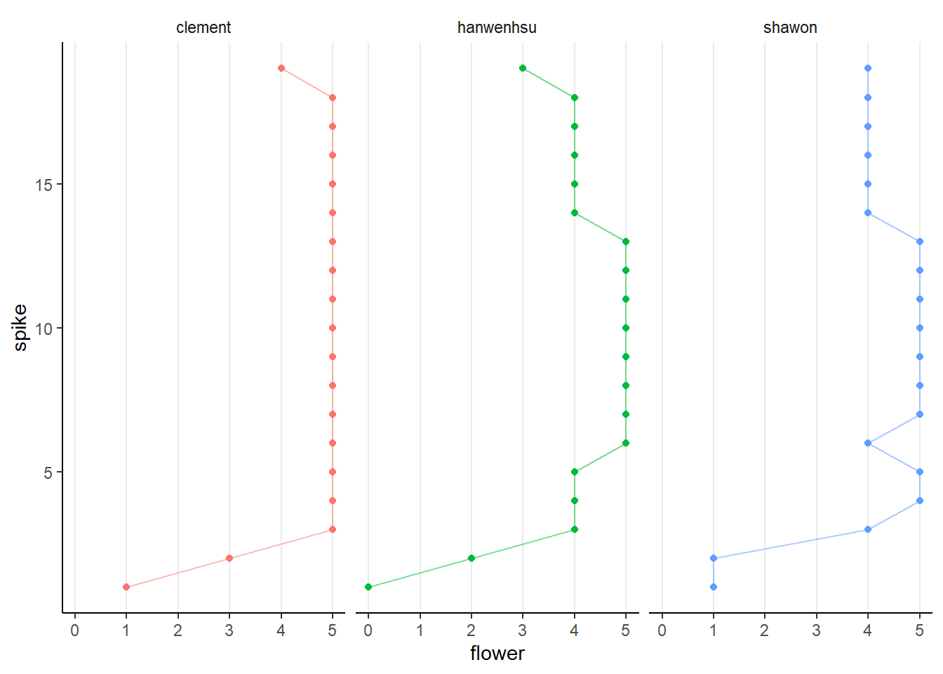
$ student      <chr> "clement", "clement", "clement", "clement", "clement", "c…

2.1 How to make it a bit more beautiful?

click for answer

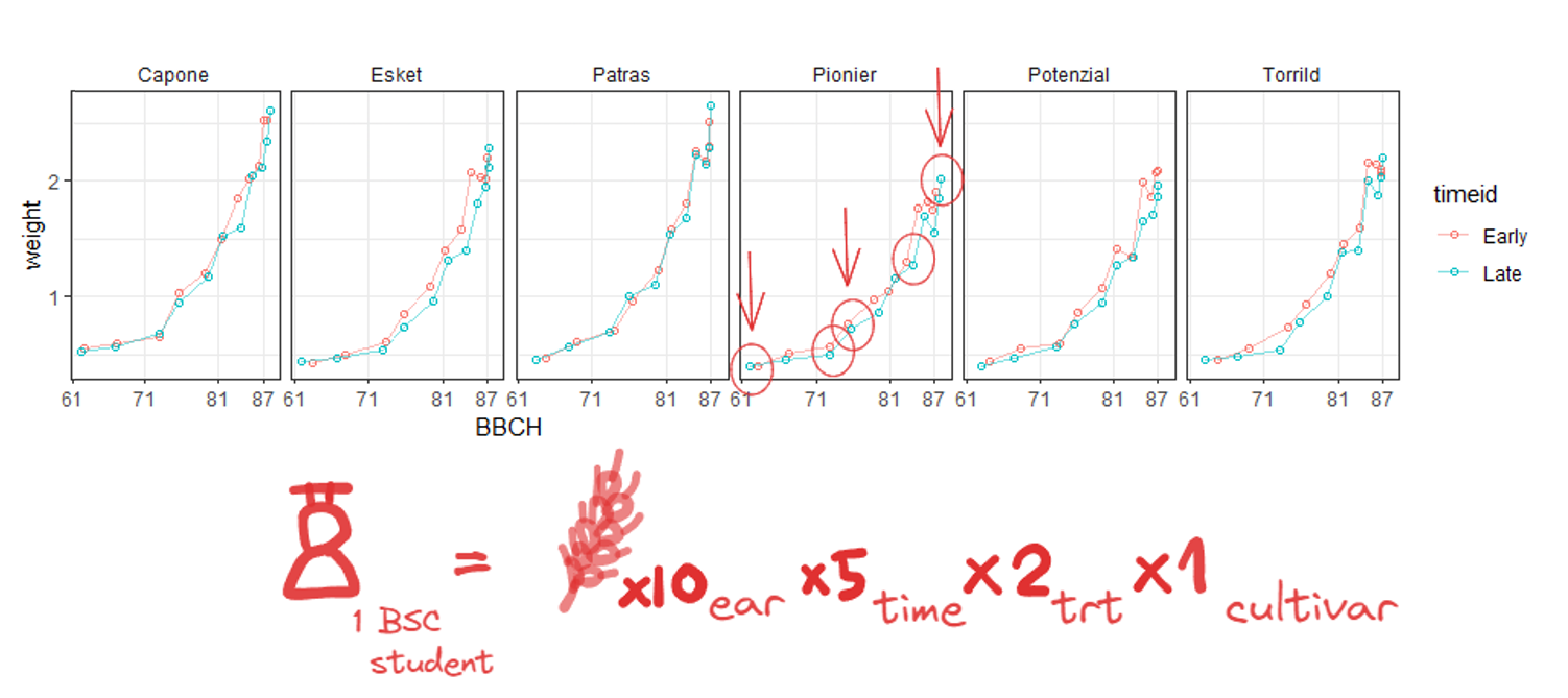
df %>% 
  group_by(student,spike) %>% 
  ggplot(aes(flower,spike,color=student))+
  geom_point()+
  geom_path(alpha=.5)+
  facet_grid(~student)+
  theme_classic()+
  theme(strip.background = element_blank(),
        panel.grid.major.x = element_line(),
        legend.position = "none")

2.2 How to place kernel-related traits in subplots?

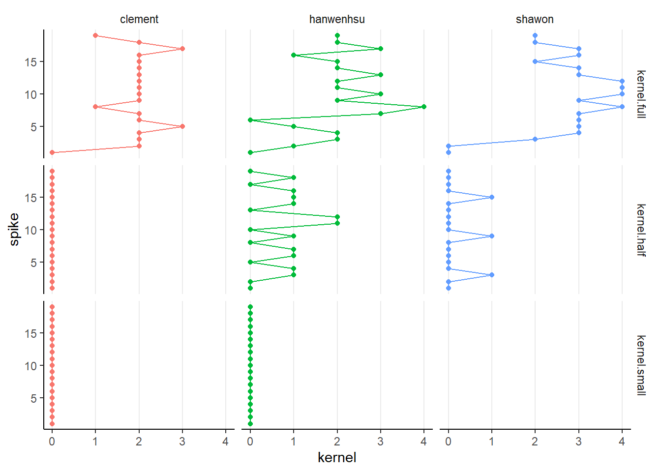
1. pivot_longer()to collect kernel-related traits
2. facet_grid()

click for answer

df %>% 
  pivot_longer(starts_with("kernel"),
               values_to = "kernel",
               names_to="kerneltype") %>% 
  group_by(student,spike) %>% 
  ggplot(aes(kernel,spike,color=student))+
  geom_point()+
  geom_path()+
  facet_grid(kerneltype~student)+
  theme_classic()+
  theme(strip.background = element_blank(),
        panel.grid.major.x = element_line(),
        legend.position = "none")

2.3 classify spikelet based on position

the spike of the main shoot was dissected to count the total number of floret in

• basal 1/3 spikelet from the bottom)

• central (middle 1/3 of spikelets)

• apical (1/3 spikelets from the top)

reference

try to clssify each spike into three classes based on their position.

challenge

1. add new column called type using mutate()
2. cut() could be useful, which column you should apply to?
3. what will you get when you pass the result of cut() to as.numeric()?
4. use case_when() to re-calssify the result of step 3.
5. based on which columns should you classify? what are your group columns for group_by?

click for answer

df %<>% 
  group_by(student,plot_id,var) %>% 
  mutate(type=cut(spike,3) %>% as.numeric(),
         type=case_when(type==1~"basal",
                        type==2~"central",
                        T~"apical"))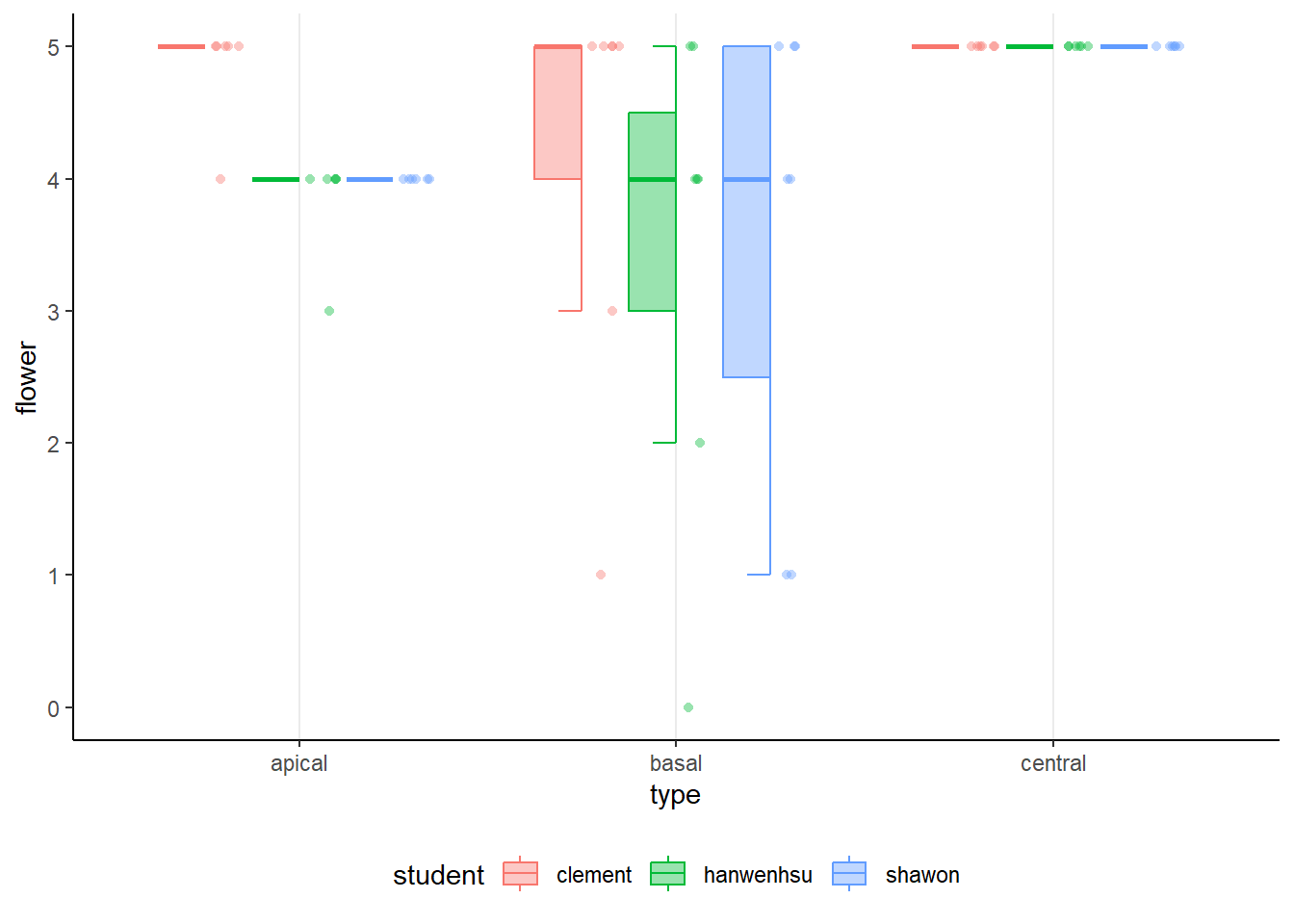

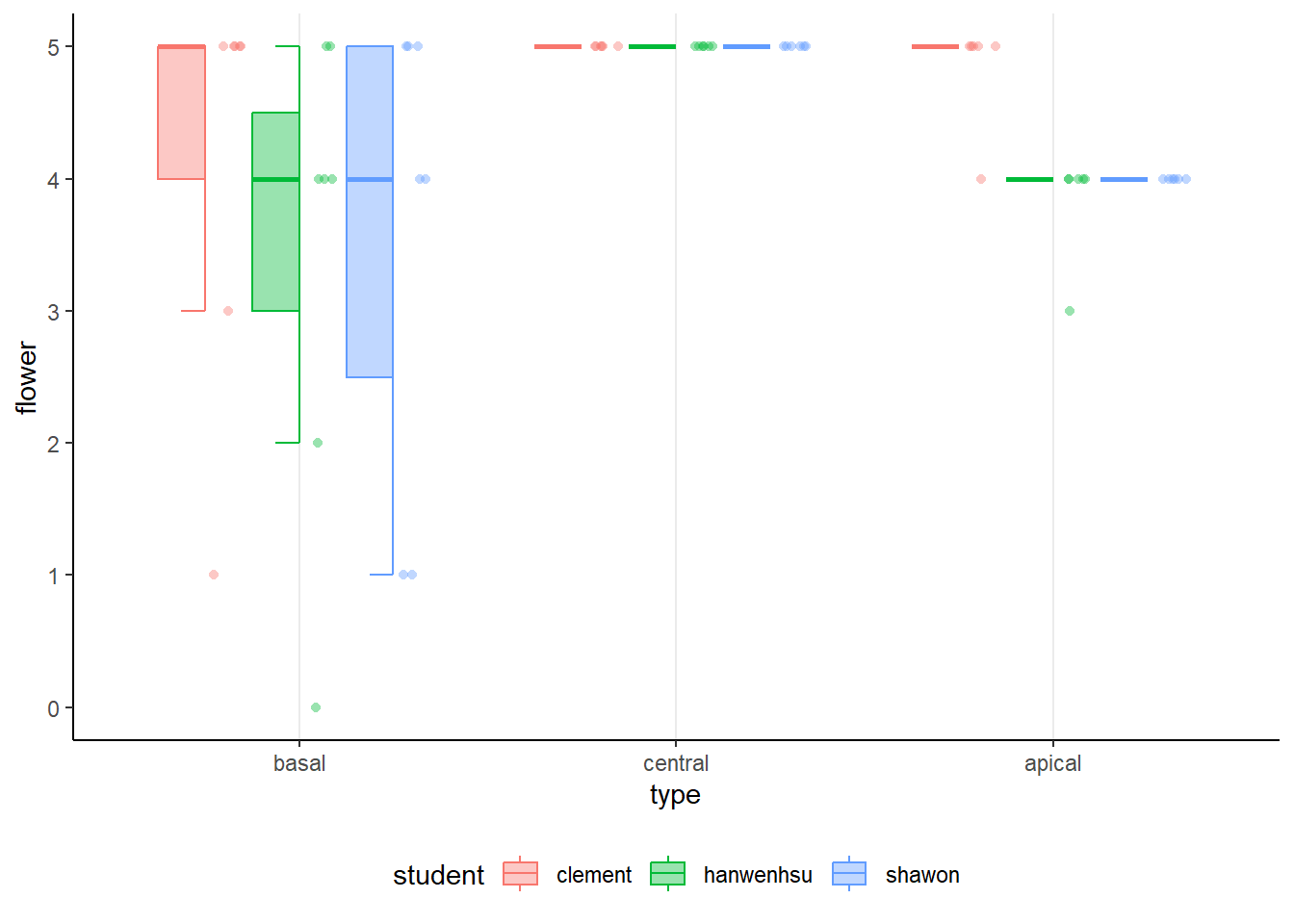
How to plot this half-box plot?

click for answer

library(ggpol)
p <- df%>% 
  ggplot(aes(type,flower,fill=student))+
  geom_boxjitter(aes(color=student),alpha=.4,
                 jitter.shape = 21, jitter.color = NA, 
                 jitter.params = list(height = 0, width = 0.04),
                 outlier.color = NA, errorbar.draw = TRUE)+
  theme_classic()+
  theme(strip.background = element_blank(),
        panel.grid.major.x = element_line(),
        legend.position = "bottom") 

print(p)

2.4 how to change the order of the box plot?

set the type as factor and arrange the levels from basal to apical.

3 recommendation

Datavisualization Scientific story telling