Week7: Shape of dataframe
R-intermediate
Welcome to the seventh course! You will learn more about dataframe wrangling:
Learning goals
- data frame wrangling with
dplyrandtidyr ggplot()
Discussion
- What is
case_when()? How to write the syntax? - When to use
match()andorder()?
Logic of coding
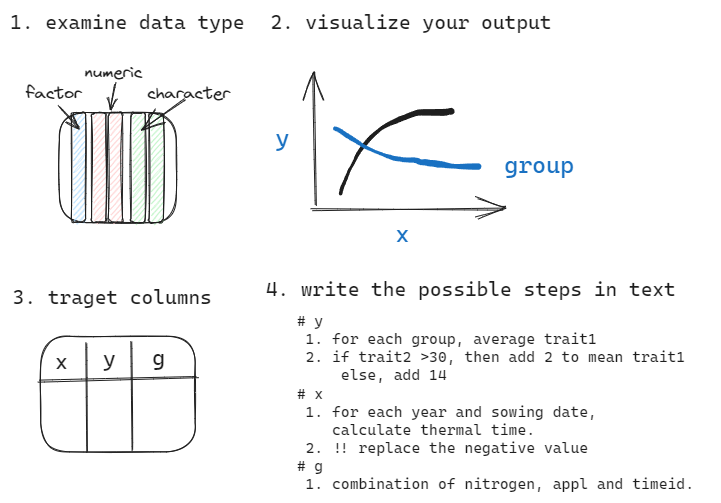
Check: examine the datatype of each column in your dataframe.
Drafting: draw the draft of your desired output.
Target columns: identify which columns you would need to generate the output.
Steps: write down the possible steps which required to generate the target columns.
challenge
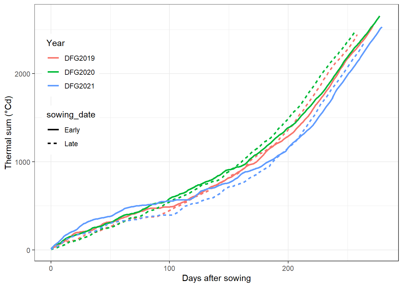
Here is a draft from coding logic step2. Please practice step 1, 3 & 4 with climate.csv. Finally, can you reproduce this figure?
answer for steps
- check the datatype of
DayTime, make sure it isDate. group_byyear and sowing date,mutatea new column calledDAS(Days after sowing).- use
ggplotto visualize this dataframe with points and lines:
x is DAS, y is Acc_Temperature, color is DFG_year and the points should be linked of same DFG_year and sowing_date.
Is there additional columns required?
answer for code
climate %>%
  # dplyr::filter(DFG_year%in%c("DFG2019","DFG2020")) %>%
  group_by(DFG_year,sowing_date) %>%
  mutate(DayTime=as.Date(DayTime,format="%Y-%m-%d"),
         DAS=as.numeric(DayTime-min(DayTime))) %>%
  ggplot(aes(x=DAS,y=Acc_Temperature,color=DFG_year,
             group=interaction(sowing_date,DFG_year)))+
  # geom_point()+
  geom_line(aes(linetype=sowing_date),linewidth=1)+
  theme_bw()+
  theme(legend.position = c(.1,.65))+
  labs(x="Days after sowing",y= "Thermal sum (°Cd)")+
  guides(color=guide_legend(title="Year"))
how to get the minimum unique combination of dataframe?
how many unique year-months combinations were included in `climate 2019 for early and late sowing?
climate %>%
  dplyr::filter(DFG_year=="DFG2019") %>%
  group_by(y,m) %>%
  summarise()

climate %>%
  dplyr::filter(DFG_year=="DFG2019") %>%
  dplyr::select(y,m) %>%
  dplyr::distinct()
challenge
read ear_summarized.csv and extract the unique combinations of nitrogen, appl and timeid
  nitrogen     appl timeid
1      176 Combined  Early
2      176 Combined   Late
3      176    Split  Early
4      176    Split   Late
5      220 Combined  Early
6      220 Combined   Late
7      220    Split  Early
8      220    Split   Late
Shapes of dataframe.
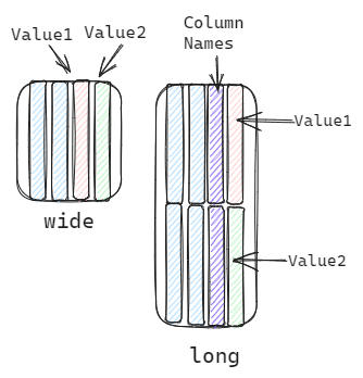
In general, we can describe the shape of dataframe as wide or long.1
Wide refers to a dataframe which each column is one trait.
Long refers to a dataframe which multiple trait names in one column and multiple trait values in another one.
Relationship of shape of dataframe and data processing
mutate() is designed for column-wise calculation.
wide format:
across()provide quick access to multiple columns, could be useful for wide format.
long format:
- Since the values are concentrated in one column, this format is suitable for unifying operation.
facet_grid()will required a column which stores the grouping information for facet. This is can be achieved via the long format.
wide to long
In the following examples, we want a unifying change
# climate %>%glimpse()
climate_long <- climate %>%
  tidyr::pivot_longer(names_to = "Daily_Terms",
                      values_to = "Daily_value",
                      cols = contains("Daily"))
# climate_long%>%   names()

#select cols by position
# grep("(Daily|Acc)",names(climate))
climate_long <- climate %>%
  tidyr::pivot_longer(names_to = "Terms",
                      values_to = "value",
                      # select both patterns
                      cols = grep("(Daily|Acc)",names(.)))

# climate_long%>% names()

## data processing example
climate_long_subset<- climate_long %>%
  filter(Terms%in%c('Acc_Temperature','Acc_Precipitation')) %>%
  group_by(DFG_year,sowing_date,Terms) %>%
  summarise(Value=mean(value))

climate_long_subset
# A tibble: 6 × 4
# Groups: DFG_year, sowing_date [6]
DFG_year sowing_date Terms Value
<chr> <chr> <chr> <dbl>
1 DFG2019 Early Acc_Temperature 923.
2 DFG2019 Late Acc_Temperature 856.
3 DFG2020 Early Acc_Temperature 1002.
4 DFG2020 Late Acc_Temperature 910.
5 DFG2021 Early Acc_Temperature 928.
6 DFG2021 Late Acc_Temperature 799.#Fig 2
library(scales) %>% suppressMessages()
climate_long %>%
filter(Terms%in%c('Acc_Temperature','Acc_Radiation'),
sowing_date=='Early') %>%
group_by(DFG_year,sowing_date) %>%
mutate(DayTime=as.Date(DayTime,format="%Y-%m-%d"),
DAS=as.numeric(DayTime-min(DayTime))) %>%
ggplot(aes(DAS,value,color=DFG_year))+
geom_line()+
facet_grid(~Terms)+
theme_test()+
theme(strip.background = element_blank(),
strip.text = element_text(size=14),
axis.text = element_text(size=14),
axis.title = element_text(size=14),
legend.position = c(.1,.1))+
scale_y_log10(
labels = label_number(scale_cut = cut_short_scale())
)+
xlab('Days after sowing')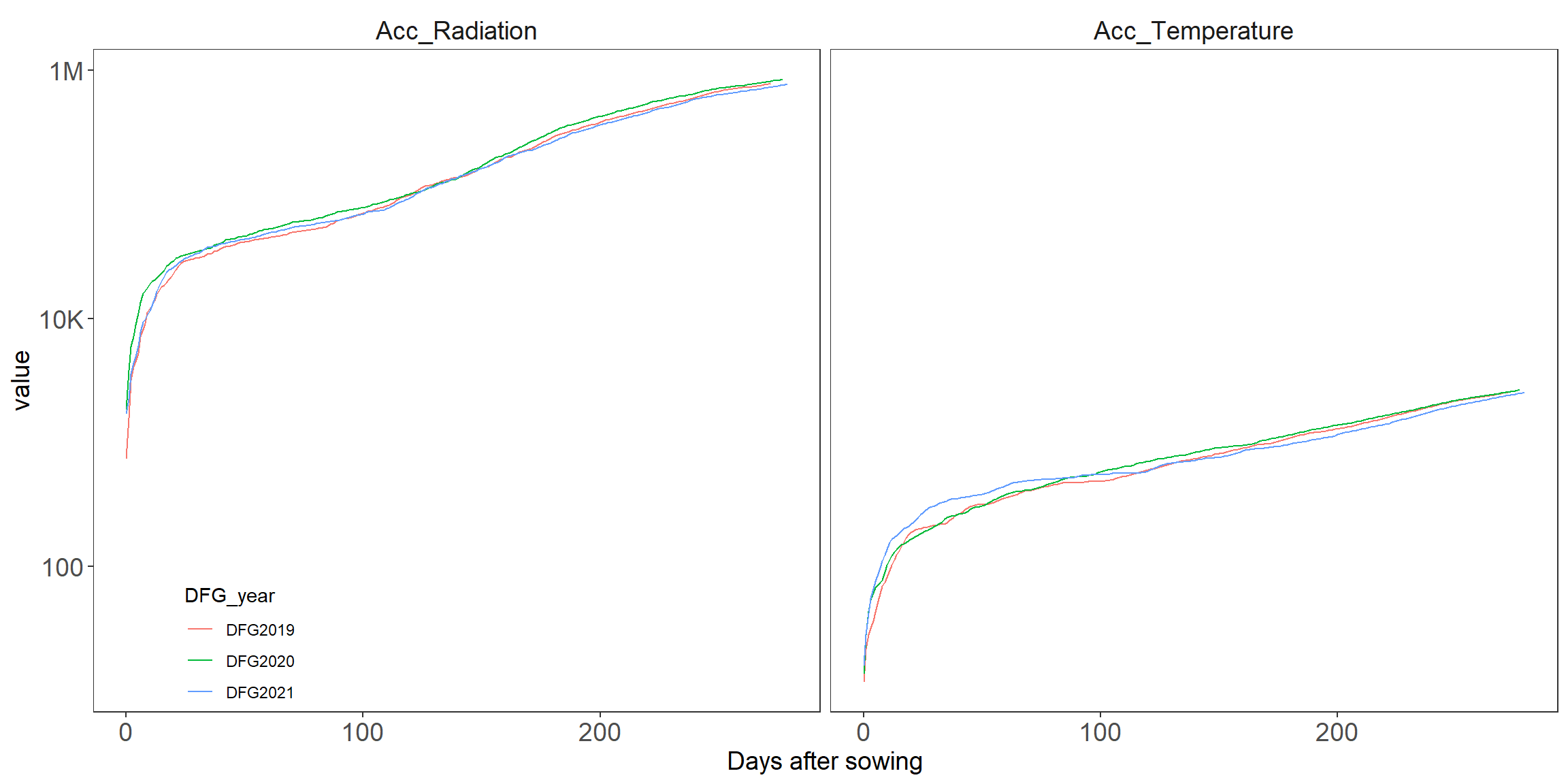
challenge
Analyze the code that generating Fig2.
Figure out how it works by blocking one line at a time. add documentation for each line.
Which function need package scales?
long ↔︎ wide
Theoretically, we can easzily switch between the forms. Are they really the same after transforming back?
# long
climate_long <- climate %>% # climate is wide
  tidyr::pivot_longer(names_to = "Daily_Terms",
                      values_to = "Daily_value",
                      cols = contains("Daily"))
# wide again
climate_wide<- climate_long%>%
  tidyr::pivot_wider(names_from = "Daily_Terms",
                     values_from = "Daily_value")

# check if they are the same
setdiff(names(climate),names(climate_wide))character(0)all.equal(climate,climate_wide) [1] "Names: 8 string mismatches"
[2] "Attributes: < Component \"class\": Lengths (1, 3) differ (string compare on first 1) >"
[3] "Attributes: < Component \"class\": 1 string mismatch >"
[4] "Component 5: Mean relative difference: 96.42546"
[5] "Component 6: Mean relative difference: 0.8220306"
[6] "Component 7: Mean relative difference: 1534.907"
[7] "Component 8: Modes: numeric, character"
[8] "Component 8: target is numeric, current is character"
[9] "Component 9: Modes: numeric, character"
[10] "Component 9: target is numeric, current is character"
[11] "Component 10: Mean relative difference: 0.9968243"
[12] "Component 11: Modes: character, numeric"
[13] "Component 11: target is character, current is numeric"
[14] "Component 12: Modes: character, numeric"
[15] "Component 12: target is character, current is numeric" # change the order of column
all.equal(climate,climate_wide[,names(climate)])[1] "Attributes: < Component \"class\": Lengths (1, 3) differ (string compare on first 1) >"
[2] "Attributes: < Component \"class\": 1 string mismatch >" # change the type
all.equal(climate,climate_wide[,names(climate)]%>% as.data.frame())[1] TRUE
Discussion
wide refers to one column one trait and long denotes the stacked traits in two columns (names and values).
From
selectandfilterpoint of view, when iswideformat useful and when islongideal?If you want to
mutatea column based on calculation between multiple traits, e.g.,DailyMean_Temperature-DailySum_Percipitation/DailySum_Radiation, then which format is more suitable? or is it both possible?
Looping with for(), lapply() and map()
deal repetitive tasks with loops.2
filename <- c('grain_counting_practice_studentName1.xlsx',
              'grain_counting_practice_studentName2.xlsx')
file_list<- filename %>% strsplit("_")
# tradition way of for loop
res <- c()
for(i in 1:2){
  res <- c(res,file_list[[i]][4])
}

# alternative in r package purrr
# chr stands for the "character" output.
purrr::map_chr(1:length(file_list),  ~{
  file_list[[.x]][4]
})

# notice that the output of map_chr must be 1 element per iteration.
purrr::map_chr(filename,  ~{
  .x %>% strsplit("_") %>% unlist()
})

# equivalent
purrr::map(filename,  ~{
  .x %>% strsplit("_") %>% unlist()
})

lapply(filename,function(x){
  x %>% strsplit("_") %>% unlist()
})
read your own data
Go to HU-box, download the student folder.
challenge
using for loop, extract the student name from file name. 1. list the files of the folder student using list.files() 2. write your own for loop. 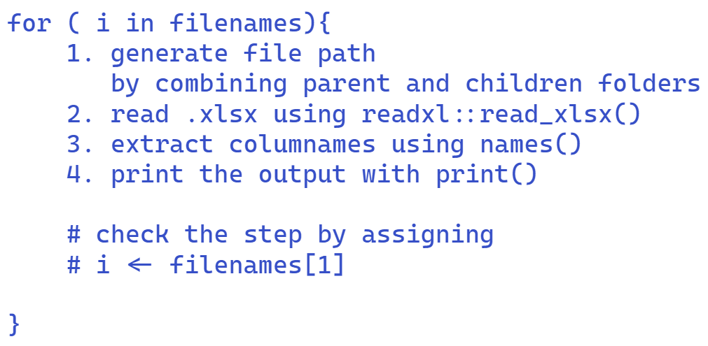
named list()